Hardware 2

This guide will provide an introduction to the design principles underpinning the drive and systems requiring actuators. We will discuss the important principles of DC motors, and how to design a system to given specifications. As part of our engineering design process, we will demonstrate how to mathematically model some of your important design considerations. The ability to develop sound mathematical models is a core element of quality engineering design. Understanding how to model a system mathematically, and how to make reasonable assumptions, provides a solid foundation toward developing a physical system that meets your design requirements. The first element of our design process involves understanding DC motor curves, which can be used to determine some important design constraints.

Understanding Motors

In this section we are going to discuss motor specifications and motor curves. We need to understand the basic motor specifications and how they translate to drawing motor curves. These motor curves will then be very useful in helping you select an appropriate motor for your application. The first motor specifications we are going to look at are the nominal voltage, the no load speed and the stall torque;

The nominal voltage is the recommend voltage the motor should operate at.
The no load speed is the maximum speed of the motor, calculated when no torque is applied to the output shaft, and when operating at the given nominal voltage.
The stall torque is the maximum torque that can be outputted by the motor, however the output shaft will no longer be in rotation.

A motor's no load speed and the stall torque are typically given based on the specified nominal voltage. What these three specifications allow us to do is draw a torque vs speed graph, as can be seen in the following figure. We typically assume the relationship between torque and speed is linear.

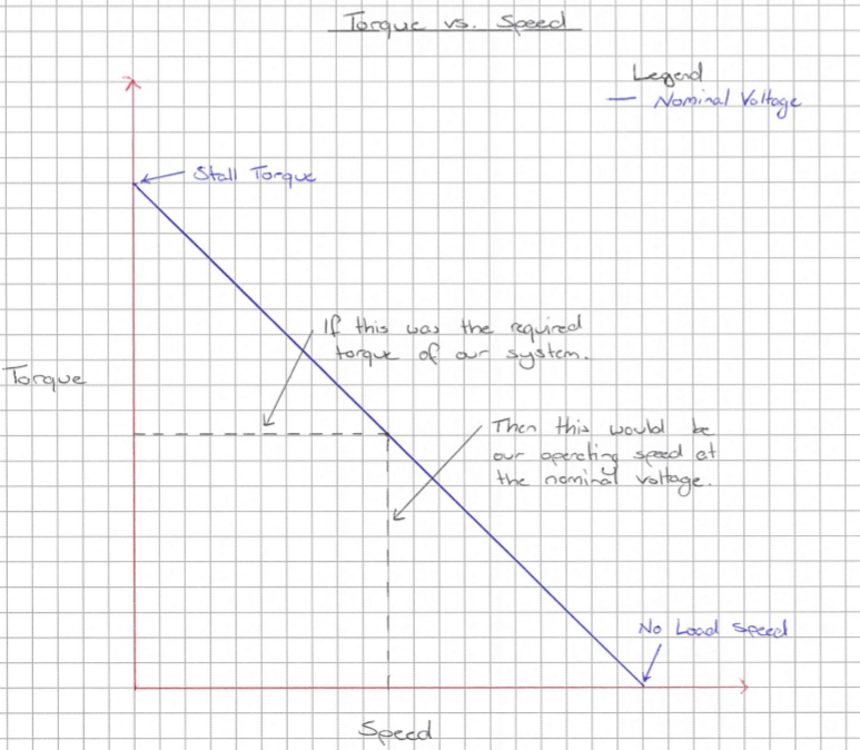
Image Not Found — An Example of a Motor Torque vs. Speed Graph and how to use one

So how do you use this graph? Well, first if we know the required motor torque to move our robot (which we will calculate later in this guide), we can read off this graph to determine the speed of the motor at the required torque, assuming operation at nominal voltage.

We do not have to operate our motor at its nominal voltage; we can supply a voltage that is higher or lower, we just have to be aware of possible operational changes. As you may know, the speed of a motor is directly proportional to the voltage applied to it. This is such that, in most cases, applying twice the voltage will double the speed. However, we must consider the low voltage alternative, since a motor does not necessarily start to spin the moment any voltage is applied. You probably have seen this in action; you need to supply above a certain voltage before the motor even starts to turn. This is because the motor needs to overcome its own internal forces before it will start rotating the output shaft. This voltage range prior to motor operation is what is known as the 'dead zone'. The following figure represents this idea graphically.

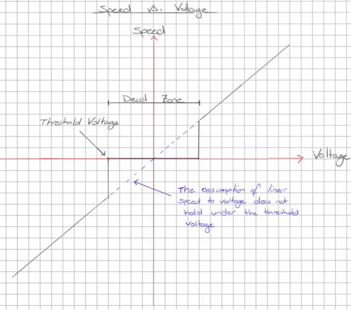
High quality motors with good datasheets may specify the dead zone, however for less expensive motors they will typically not give you this value. You will therefore need to assume a threshold voltage, which may be anywhere between 20-50% of the nominal voltage.

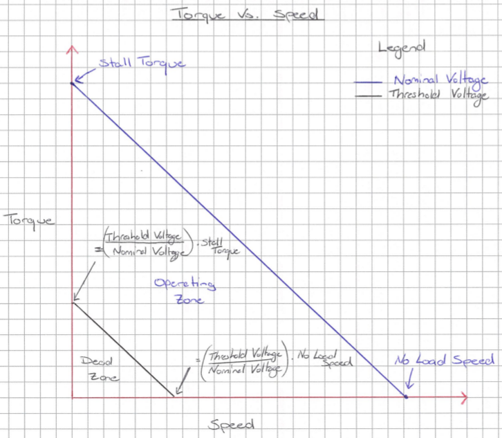
Now we can actually translate this dead zone threshold voltage onto the motor torque vs. speed graph. We can do this by making the assumption that the speed and torque are proportional to the voltage. This is such that if we halve the operating voltage then we will get half the torque and half the speed. So we can draw a line on our motor torque vs speed graph to represent the threshold voltage. This allows us to visualize the motor operating zone, as can be seen in the figure below.

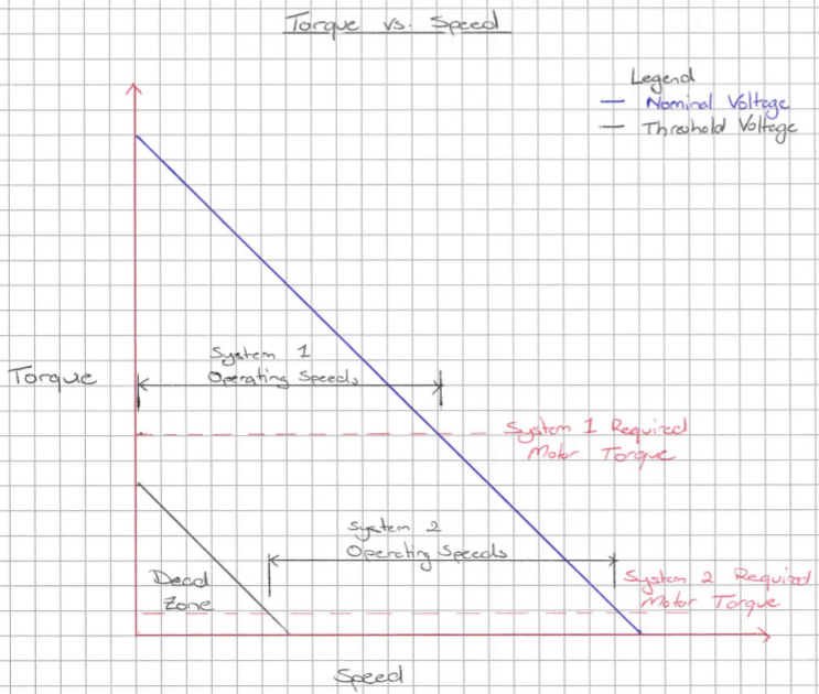
We can use this graph similarly to the graph we examined earlier. If our required motor torque is plotted as a horizontal line, we can visually see what the motor's speed will be at various voltages (the voltage decreases as we move from the nominal voltage toward the y-axis). On the graph below we show two different required motor torque examples; you should notice one of our horizontal torque lines ends up in the dead zone and so we could not acheive low speeds.

A motor can also operate above its nominal voltage, and we can add this to the motor torque vs. speed graph as well. However, you must be careful when operating at voltages significantly higher than the nonimal voltage or extremely close to the threshold voltage. Operating near these points can drastically reduce the lifetime of your motor. It can also destroy electronic circuits if they have not been designed to withstand these voltage levels and the high current induced by operating in these zones.

Now that we understand the basic motor curves, and how we can generate them, we can start to look at designing our various systems.

Designing a Drive System

Design Requirements

Typically when designing a drive system we are trying achieve certain velocities and a minimum acceleration. To achieve these velocity and acceleration profiles, we need to consider our application and select appropriate motors and wheel sizes while considering the robot parameters, particularly the robots mass.

For this example we are going to be designing a medium-sized differential drive robot that will be used by researchers to perform outdoor place recognition experiments. The terrain will be mainly flat, and the researchers want the robot to be able to achieve a speed that is equal to or greater than human walking speed (5km/hr). You should also remember that the velocities and acceleration you need to factor into your design are dependent on the application.

So first we need to define our operating velocities as well as our minimum acceleration. The researchers have provided us with the the minimum top speed which is approximately 1.5m/s. From this minimum top speed we can also reason a suitable minimum acceleration. We can do this by deciding how quickly we want our robot to be able to achieve this top speed. For this example, let's say it needs to reach 1.5m/s in 2 seconds; so we have a minimum acceleration of 0.75m/s^2. The final piece of the puzzle is the maximum low speed; we want our robot to be capable of moving at speeds below this threshold. Depending on your application, you may not need a maximum low speed, however for this example we do need to consider this factor as we want our robot to be able to move at speeds less than 0.2m/s.

To recap we have decided on 3 engineering design requirements:

Minimum Acceleration: 0.75 m/s^2
Minimum Top Speed: 1.5m/s
Maximum Low Speed: 0.2m/s

Drawing a Free Body Diagram

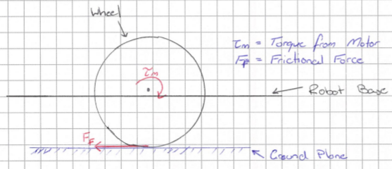
The next step in our process is to draw a free body diagram. We are going to draw the side view of our differential drive robot and we are going to make the assumption the centre of mass of the robot is directly above the center of the wheel axle. From the free body diagram below, you can see that in our very simple model we only have two forces acting on the robot's wheels; the torque from the motor, and the force due to friction.

Developing a Mathematical Model

We now need to develop a mathematical model of our drive system. This will involve using physics knowledge to somehow relate the forces in our free body diagram with our design requirements, allowing the selection of a suitable motor. To start, we need to remember Newton's second law: the cumulative force exterted on an object is equal to its mass multipled by its acceleration, or mathematically ΣF = ma. From our free body diagram we can mathematically determine the required output torque for a desired acceleration:

ΣF = m_r * a
2*(τ_o⁄r_w) - 2*F_f = m_r * a
τ_o = (0.5 * m_r * a + F_f) * r_w

The torque and friction force terms are multiplied by 2 because we have two wheels on our differential drive robot and we must include all forces acting on our robot. Using our knowledge of physics, we can determine the frictional force. The force due to friction is a product of the normal force multipled by a coefficient of friction. If we assume the robot is operating on flat surface parallel to the ground, we can state that the normal force is equal to half the robot's mass times gravity. Why half the robot's mass? Well remember we have two drive wheels and we assumed the center of mass is directly above the wheels and halfway between them, so each wheel will "support" half the mass. Hence, we can say that the required output torque for a given acceleration is given by the following equation:

τ_o = (0.5 * m_r * a + F_f) * r_w
τ_o = (0.5 * m_r * a + μ * N_f) * r_w
τ_o = (0.5 * m_r * a + 0.5 * μ * m_r * g) * r_w
τ_o = (0.5 * m_r * r_w) * (a + μ * g)

Now, as engineers we are also aware of a little thing called loss. Throughout the drive system there are going to be losses. These losses could be due to heat, or noise, and caused by friction in the gears, or the shaft spinning within the wheel hub. Simply put, the power that we put in is not going to be the power we get out, and so we can model this as an efficiency factor. The required output torque is the torque we need at the wheel itself, which will only be a percentage of the torque supplied by the motor. Hence, mathematically:

τ_output = η * τ_motor

If we substitute this into our required output torque equation, and rearrange, we can obtain our final equation. This final equation specifies the required motor torque given a desired acceleration, and some design parameters such as wheel radius for a two wheel differential drive robot.

τ_m = (1⁄η) * (0.5 * m_r * r_w) * (a + μ * g)		# Equation 2.1

From the formulas above you can also see we require the mass of the robot, the radius of the robot's drive wheels, a coefficient of friction, and an efficiency. Obviously you do not currently have these, but they are what are sometimes referred to as design parameters. These design parameters are values that you may be able to change in order to tailor your design to the design requirements. For example, we could change the wheel radius, which would subsequently affect the acceleration and top speed of our robot. Additionally, some of these design parameters may become design requirements. For example, after performing all our calculations and selecting a motor we may consider the mass of the robot to be a design requirement; as in we must ensure the mass of robot does not exceed this value.

We need to relate our velocity design requirements with our robot design parameters. In this case we do not need a free body diagram, we only need to know that linear velocity is equal to angular velocity multipled by the radius (v = ωr). So our minimum top speed and maximum top speed in terms of our design parameters are given by:

ω_min = v_min ⁄ r_w						# Equation 2.2
ω_max = v_max ⁄ r_w						# Equation 2.3

Choosing Initial Design Parameters and Calculating Motor Values

We will now work out 4 parameters, using Equations 2.1, 2.2 and 2.3, that will help us select a motor. These parameters are:

The motor torque required to overcome friction (i.e. acceleration equals 0). This is the required torque to maintain a given speed. We will call this the Friction Torque.
The motor torque required to accelerate given our acceleration design requirement. We will denote this as the Acceleration Torque.
The top motor speed. We will denote this as the Top Motor Speed.
The low motor speed. We will call this the Low Motor Speed.

However, first we will need to obtain some initial values for our design parameters (some of which may come from the design requirements). For this example we have selected the following:

Robot Mass: 10kg
Wheel Radius: 0.04m
Coefficient of Friction: 0.9
Efficiency: 0.8

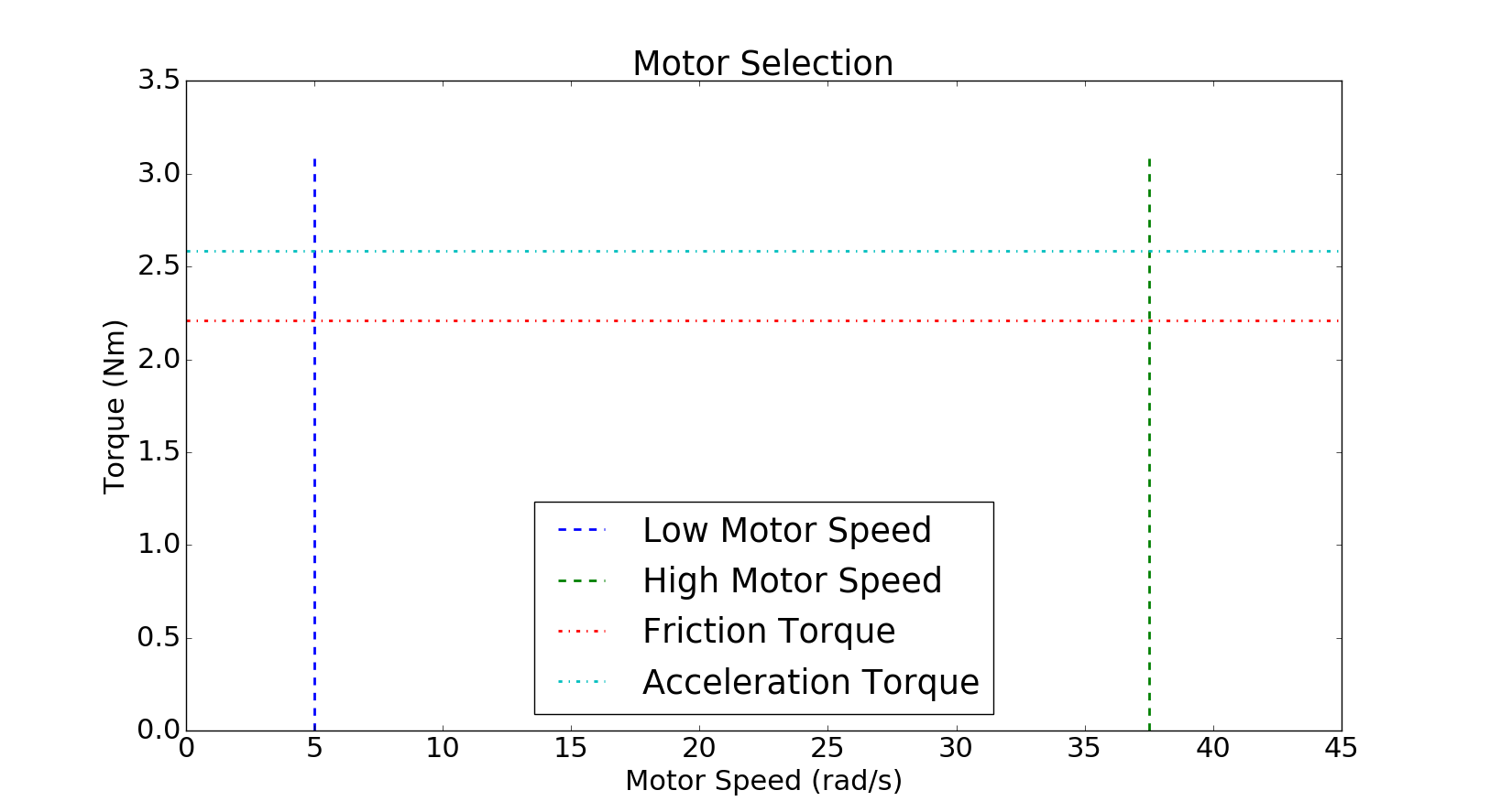
Using these values alongside our design requirements we calculate the 4 parameters to be:

Friction Torque = 2.207 Nm
Acceleration Torque = 2.395 Nm
High Motor Speed = 37.5 rad/s
Low Motor Speed = 5 rad/s

Selecting a Motor

We can now use the 4 parameters calculated in the previous section to help us select a motor. To start, we are going to draw these parameters as 2 horizontal and 2 vertical lines on a torque vs speed graph.

So now we need to traverse our favourite motor suppliers and attempt to find a suitable motor. For this example, we found a DC brushed motor with the following characteristics:

Nominal Voltage: 24 V
Motor Stall Torque: 3 Nm
Motor No Load Speed: 450 RPM
Stall Current: 5.8 A

Using these values we can plot the nominal and threshold voltage torque vs. speed curves on the same graph as our calculated design parameters, as shown in the figure below. Unfortunately, the motor datasheet did not state the threshold voltage or give us any information that allows us to approximate it, so we are going to set the threshold voltage to be approximately 40% of the nominal voltage.

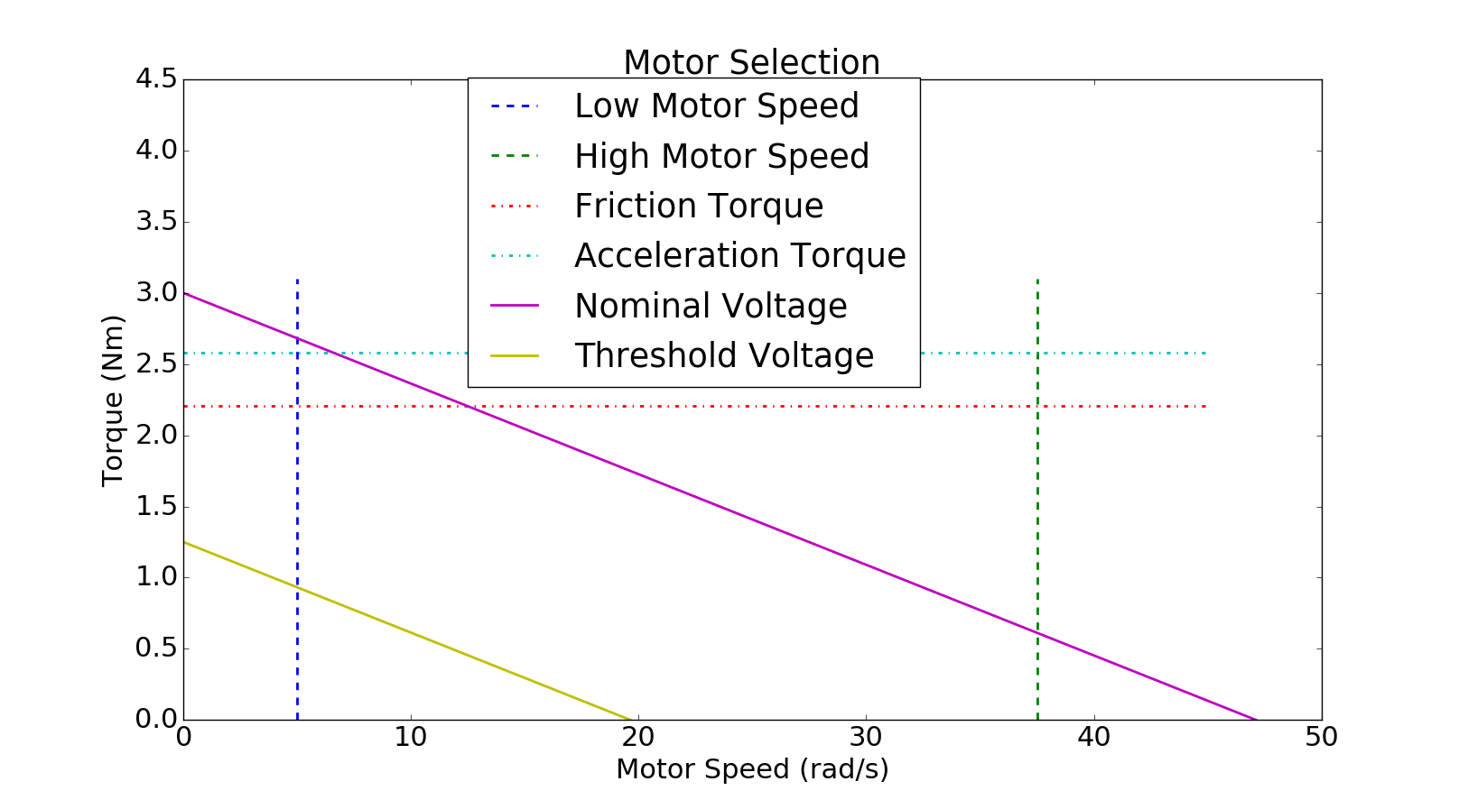
From this graph, we now need to investigate two particular critical points; these being the intersection of the Friction Torque line with each of the Low and High Motor Speed lines. We need to ensure that these intersection points are within our operating zone. As we can see from the graph, only our low motor speed intersection point is within our operating zone and this motor is probably not suitable for our application. While we could run the motors at a higher voltage to try and achieve the high motor speed; we would need to run them at approximately double the nominal voltage which would drastically reduce the motor's lifetime. However, from this graph we can intuitively see that if we could get a motor with a bit more torque and a higher RPM, we should be able to meet our design requirements. So we do some more searching and find the following motor:

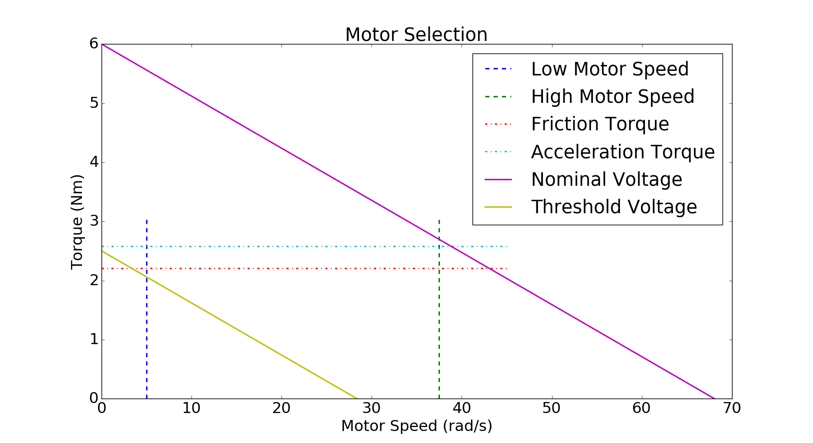
Nominal Voltage: 24 V
Motor Stall Torque: 6 Nm
Motor No Load Speed: 650 RPM
Stall Current: 16.7 A

By plotting this motor's torque vs. speed graph and overlaying the calculated design values we can see that this motor could be suitable, as shown in the figure below. The first thing we notice is that our friction torque line intersects with our high and low motor speed lines within the operating zone. This means that the motor should be able to achieve our desired minimum and maximum forward velocities. The next thing we shoud take note of is that our acceleration torque line is well below the stall torque, so we should be able to achieve our desired minimum acceleration. While this motor appears to be suitable for our application, the low motor speed and friction torque intersection point is quite close to our threshold voltage. This means that if our models and assumptions are slightly off then we may not be able to achieve our desired low forward velocity.

Okay so we have now selected our motors, what next? Well next we would need to ensure that the weight of the motor and its stall current are suitable for our system. If they are, we would then need to go design the motor driver circuitry in order to control this motor. A tip for selecting a H-Bridge IC; make sure you get a H-Bridge with in-built under-voltage, over-current and over-temparature protection. It may cost you a little bit more, but it will save you a lot of issues. Additionally, make sure the H-Bridge can handle more than the stall current specified by the motor.

Stability Analysis

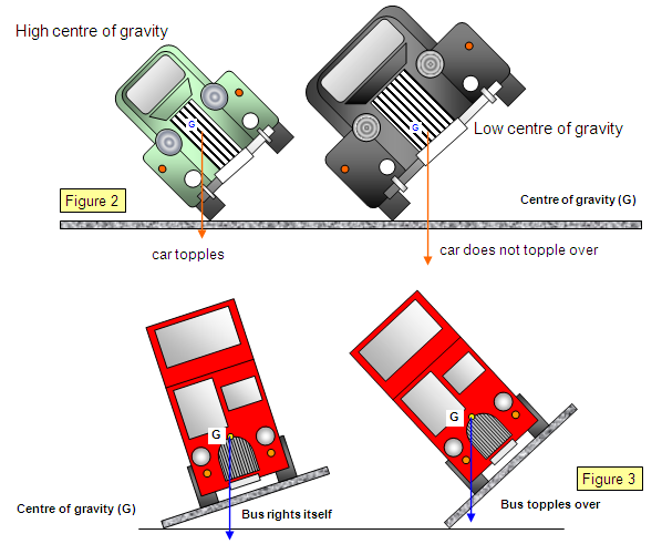
In this section we are going to perform a basic stability analysis, identifying the angle required to tip over a rock. A stability analysis looks at what angle will cause the gravity vector to move outside the limits of the platform, see the following figure for some examples.

To perform a stability analysis we require the Center of Mass (COM) of an object. We need the COM of an object as we assume the gravity vector will pass through this point. There are many ways to identify the COM of an object, for more information check out this Khan Academy article. We are going to perform a stability analysis on the lunar project rocks, assuming that the COM is at the center of the rock. This assumption probably does not hold due to the cut-outs in the bottom of the rock, but you would need to validate/invalidate this assumption yourself.

In the figure below you can see a side view of our rock, assumed to be a simple cube. To identify the tipping angle we need to identify the angle at which the gravity vector will be pass outside the object. We can do this by identifying the angle at which the gravity vector will point towards one of our corners, which will require some basic trignometry. Firstly, We know the side length (L) and we can use this to identify the angle phi (φ) and in turn angle theta (θ)

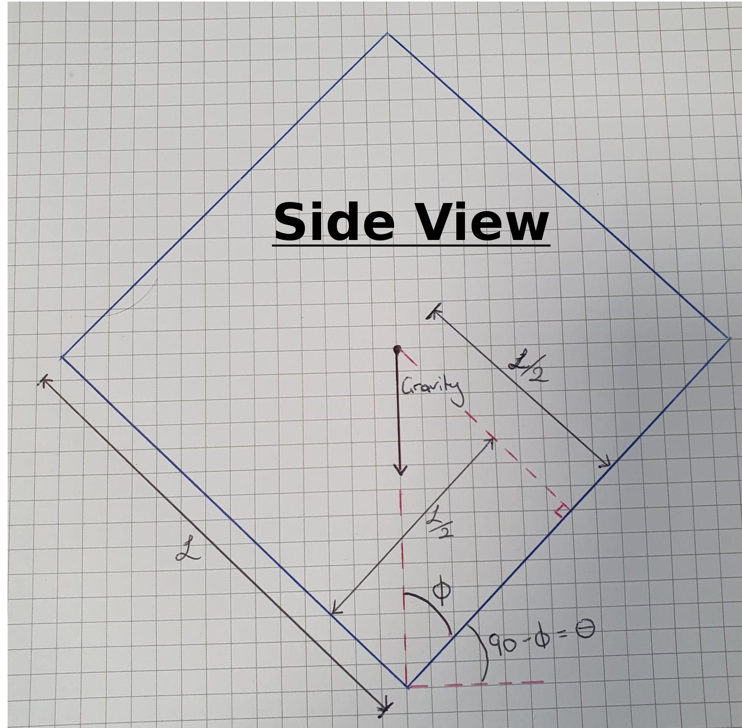
So the angle φ will be given by,

φ = atan((L/2)/(L/2)
φ = π/4 = 45°

Theta is then simply,

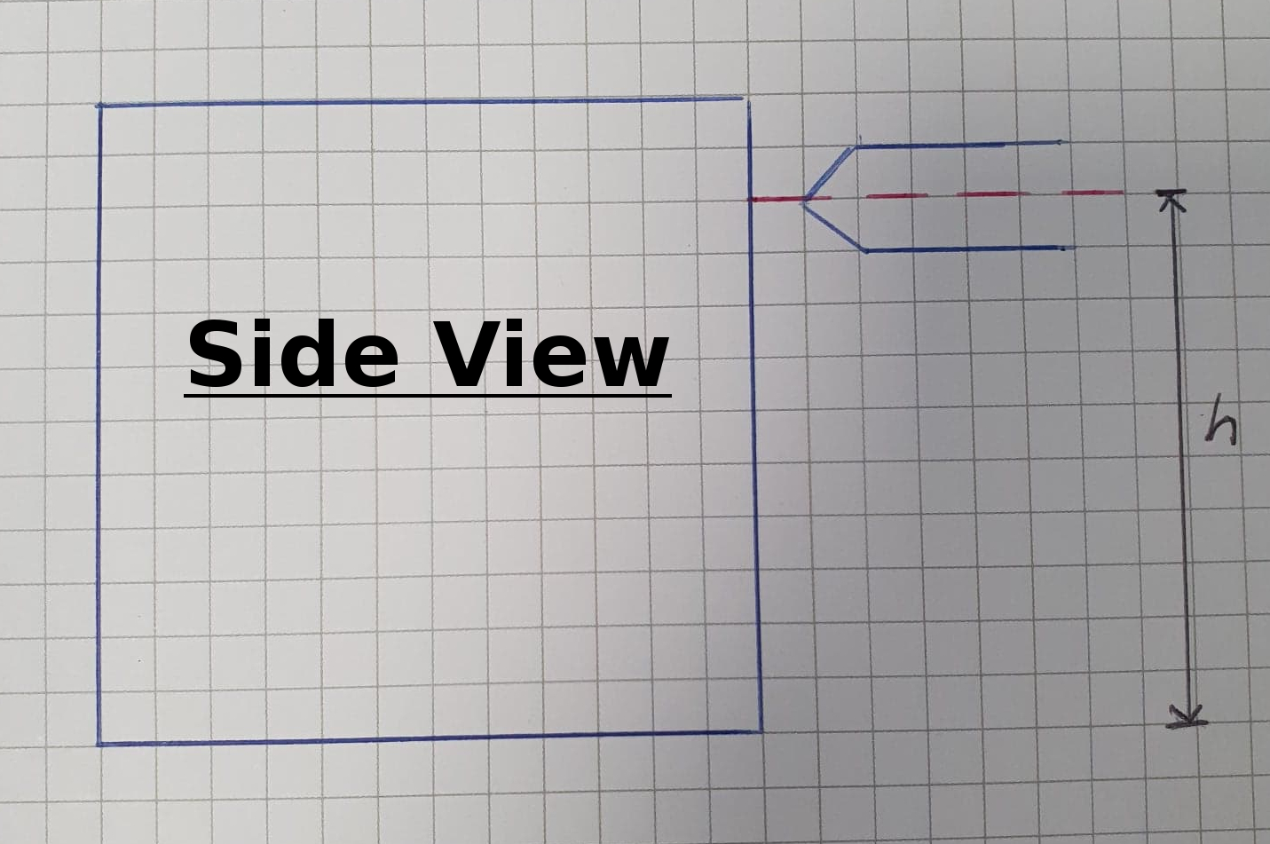
θ = π/4 = 45°

So once the block is at an angle greater than 45°, relative to the ground, it will tip over. We can utilise this information to help us design a system to topple the rock. In this example, we will investigate a system that will push the rock. A critical design parameter of this pushing system will be determining the stroke length required to tip the rock over. The height of our pushing device, relative to the ground, will be given by the letter h, which is a design parameter you can play with which will affect the stroke length required.

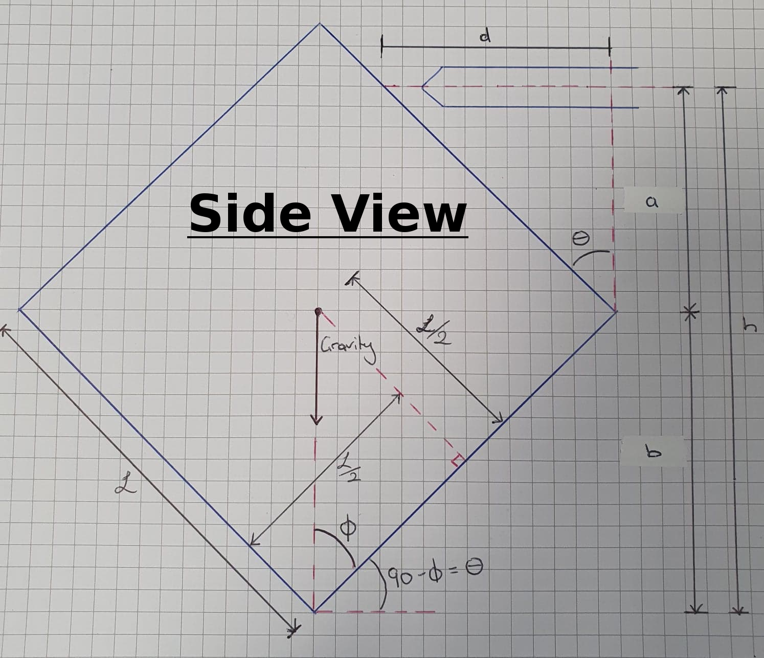
To determine the required stroke length, given by d, we need some more trignometry as well as the identified rock tipping angle of 45°. To calculate d, the stroke length, we need the length of variable a which in turn requires the length of variable b. Variable b is given by,

b = L*sin(θ)

Now given that our pushing rod is at height h, we can work out variable a

a = h - b
a = h - L*sin(θ)

Now that we know variable a, we can determine the stroke length, d,

d = a*tan(θ)
d = (h - L*sin(θ))*tan(θ)

Now we have a formula for the required stroke length of our tipping device. This formula is only dependent on the height of the pushing rod, a design parameter; the value of L and θ are given/calculated by the size of the rock and its center of mass. Remember we have made an assumption that the rock would pivot at the opposite base corner, this may not be true and some experimentation would be required to see if this is valid.